RNAmodR: analyzing high throughput sequencing data for post-transcriptional RNA modification footprints
Felix G.M. Ernst and Denis L.J. Lafontaine
2025-09-23
Source:vignettes/RNAmodR.Rmd
RNAmodR.RmdIntroduction
Post-transcriptional modifications can be found abundantly in rRNA and tRNA and can be detected classically via several strategies. However, difficulties arise if the identity and the position of the modified nucleotides is to be determined at the same time. Classically, a primer extension, a form of reverse transcription (RT), would allow certain modifications to be accessed by blocks during the RT or changes in the cDNA sequences. Other modification would need to be selectively treated by chemical reactions to influence the outcome of the reverse transcription.
With the increased availability of high throughput sequencing, these classical methods were adapted to high throughput methods allowing more RNA molecules to be accessed at the same time. With these advances post-transcriptional modifications were also detected on mRNA. Among these high throughput techniques are for example Pseudo-Seq (Carlile et al. 2014), RiboMethSeq (Birkedal et al. 2015) and AlkAnilineSeq (Marchand et al. 2018) each able to detect a specific type of modification from footprints in RNA-Seq data prepared with the selected methods.
Since similar pattern can be observed from some of these techniques, overlaps of the bioinformatical pipeline already are and will become more frequent with new emerging sequencing techniques.
RNAmodR implements classes and a workflow to detect
post-transcriptional RNA modifications in high throughput sequencing
data. It is easily adaptable to new methods and can help during the
phase of initial method development as well as more complex
screenings.
Briefly, from the SequenceData, specific subclasses are
derived for accessing specific aspects of aligned reads, e.g. 5’-end
positions or pileup data. With this a Modifier class can be
used to detect specific patterns for individual types of modifications.
The SequenceData classes can be shared by different
Modifier classes allowing easy adaptation to new
methods.
## No methods found in package 'rtracklayer' for request: 'trackName<-' when loading 'AnnotationHubData'## Warning: replacing previous import 'utils::findMatches' by
## 'S4Vectors::findMatches' when loading 'ExperimentHubData'
library(rtracklayer)
library(Rsamtools)
library(GenomicFeatures)
library(txdbmaker)
library(RNAmodR.Data)
library(RNAmodR)
SequenceData
Each SequenceData object is created with a named
character vector, which can be coerced to a BamFileList, or
named BamFileList. The names must be either “treated” or
“control” describing the condition the data file belongs to. Multiple
files can be given per condition and are used as replicates.
annotation <- GFF3File(RNAmodR.Data.example.gff3())
sequences <- RNAmodR.Data.example.fasta()
files <- c(Treated = RNAmodR.Data.example.bam.1(),
           Treated = RNAmodR.Data.example.bam.2(),
           Treated = RNAmodR.Data.example.bam.3())
For annotation and sequences several input
are accepted. annotation can be a GRangesList,
a GFF3File or a TxDb object. Internally, a
GFF3File is converted to a TxDb object and a
GRangesList is retrieved using the exonsBy
function.
seqdata <- End5SequenceData(files, annotation = annotation,
                            sequences = sequences)
## Import genomic features from the file as a GRanges object ... OK
## Prepare the 'metadata' data frame ... OK
## Make the TxDb object ...## Warning in .makeTxDb_normarg_chrominfo(chrominfo): genome version information
## is not available for this TxDb object## OK
## Loading 5'-end position data from BAM files ... OK
seqdata## End5SequenceData with 60 elements containing 3 data columns and 3 metadata columns
## - Data columns:
## end5.treated.1 end5.treated.2 end5.treated.3
## <integer> <integer> <integer>
## - Seqinfo object with 84 sequences from an unspecified genome; no seqlengths:SequenceData extends from a
CompressedSplitDataFrameList and contains the data per
transcript alongside the annotation information and the sequence. The
additional data stored within the SequenceData can be
accessed by several functions.
names(seqdata) # matches the transcript names as returned by a TxDb object
colnames(seqdata) # returns a CharacterList of all column names
bamfiles(seqdata)
ranges(seqdata) # generate from a TxDb object
sequences(seqdata)
seqinfo(seqdata)
Currently the following SequenceData classes are
implemented:
End5SequenceDataEnd3SequenceDataEndSequenceDataProtectedEndSequenceDataCoverageSequenceDataPileupSequenceDataNormEnd5SequenceDataNormEnd3SequenceData
The data types and names of the columns are different for most of the
SequenceData classes. As a naming convenction a descriptor
is combined with the condition as defined in the files input and the
replicate number. For more details please have a look at the man pages,
e.g. ?End5SequenceData.
SequenceData objects can be subset like a
CompressedSplitDataFrameList. Elements are returned as a
SequenceDataFrame dependent of the type of
SequenceData used. For each SequenceData class
a matching SequenceDataFrame is implemented.
seqdata[1]## End5SequenceData with 1 elements containing 3 data columns and 3 metadata columns
## - Data columns:
## end5.treated.1 end5.treated.2 end5.treated.3
## <integer> <integer> <integer>
## - Seqinfo object with 84 sequences from an unspecified genome; no seqlengths:
sdf <- seqdata[[1]]
sdf
## End5SequenceDataFrame with 1649 rows and 3 columns
## end5.treated.1 end5.treated.2 end5.treated.3
## <integer> <integer> <integer>
## 1 1 4 0
## 2 0 2 0
## 3 0 0 0
## 4 0 0 0
## 5 0 0 0
## ... ... ... ...
## 1645 0 0 0
## 1646 0 0 0
## 1647 0 0 0
## 1648 0 0 0
## 1649 0 0 0
##
## containing a GRanges object with 1 range and 3 metadata columns:
## seqnames ranges strand | exon_id exon_name exon_rank
## <Rle> <IRanges> <Rle> | <integer> <character> <integer>
## [1] Q0020_15S_RRNA 1-1649 + | 1 Q0020 1
## -------
## seqinfo: 60 sequences from an unspecified genome; no seqlengths
##
## and a 1649-letter RNAString object
## seq: GUAAAAAAUUUAUAAGAAUAUGAUGUUGGUUCAGAU...UGCGGUGGGCUUAUAAAUAUCUUAAAUAUUCUUACAThe SequenceDataFrame objects retains some accessor
functions from the SequenceData class.
Subsetting of a SequenceDataFrame returns a
SequenceDataFrame or DataFrame, depending on
whether it is subset by a column or row, respectively. The
drop argument is ignored for column subsetting.
sdf[,1:2]## End5SequenceDataFrame with 1649 rows and 2 columns
## end5.treated.1 end5.treated.2
## <integer> <integer>
## 1 1 4
## 2 0 2
## 3 0 0
## 4 0 0
## 5 0 0
## ... ... ...
## 1645 0 0
## 1646 0 0
## 1647 0 0
## 1648 0 0
## 1649 0 0
##
## containing a GRanges object with 1 range and 3 metadata columns:
## seqnames ranges strand | exon_id exon_name exon_rank
## <Rle> <IRanges> <Rle> | <integer> <character> <integer>
## [1] Q0020_15S_RRNA 1-1649 + | 1 Q0020 1
## -------
## seqinfo: 60 sequences from an unspecified genome; no seqlengths
##
## and a 1649-letter RNAString object
## seq: GUAAAAAAUUUAUAAGAAUAUGAUGUUGGUUCAGAU...UGCGGUGGGCUUAUAAAUAUCUUAAAUAUUCUUACA
sdf[1:3,]## DataFrame with 3 rows and 3 columns
## end5.treated.1 end5.treated.2 end5.treated.3
## <integer> <integer> <integer>
## 1 1 4 0
## 2 0 2 0
## 3 0 0 0Modifier
Whereas, the SequenceData classes are used to hold the
data, Modifier classes are used to detect certain features
within high throughput sequencing data to assign the presence of
specific modifications for an established pattern. The
Modifier class (and its nucleotide specific subclasses
RNAModifier and DNAModifier) is virtual and
can be addapted to individual methods. For example mapped reads can be
analyzed using the ModInosine class to reveal the presence
of I by detecting a A to G conversion in normal RNA-Seq data. Therefore,
ModInosine inherits from RNAModifier.
To fix the data processing and detection strategy, for each type of
sequencing method a Modifier class can be developed
alongside to detect modifications. For more information on how to
develop such a class and potentially a new corresponding
SequenceData class, please have a look at the vignette for creating a new
analysis.
For now three Modifier classes are available:
ModInosine-
ModRiboMethSeqfrom theRNAmodR.RiboMethSeqpackage -
ModAlkAnilineSeqfrom theRNAmodR.AlkAnilineSeqpackage
Modifier objects can use and wrap multiple
SequenceData objects as elements of a
SequenceDataSet class. The elements of this class are
different types of SequenceData, which are required by the
specific Modifier class. However, they are required to
contain data for the same annotation and sequence data.
Modifier objects are created with the same arguments as
SequenceData objects and will start loading the necessary
SequenceData objects from these. In addition they will
automatically start to calculate any additional scores (aggregation) and
then start to search for modifications, if the optional argument
find.mod is not set to FALSE.
mi <- ModInosine(files, annotation = annotation, sequences = sequences)## Import genomic features from the file as a GRanges object ... OK
## Prepare the 'metadata' data frame ... OK
## Make the TxDb object ...## Warning in .makeTxDb_normarg_chrominfo(chrominfo): genome version information
## is not available for this TxDb object## OK
## Loading Pileup data from BAM files ... OK
## Aggregating data and calculating scores ... Starting to search for 'Inosine' ... done.(Hint: If you use an artificial genome, name the chromosomes
chr1-chrN. It will make some things easier for subsequent visualization,
which relies on the Gviz package)
Since the Modifier class wraps a
SequenceData object the accessors to data contained within
work similarly to the SequenceData accessors described
above. What type of conditions the Modifier class
expects/supports is usually described in the man pages of the Modifier
class.
names(mi) # matches the transcript names as returned by a TxDb object
bamfiles(mi)
ranges(mi) # generated from a TxDb object
sequences(mi)
seqinfo(mi)
sequenceData(mi) # returns the SequenceData
Settings
The behavior of a Modifier class can be fine tuned using
settings. The settings() function is a getter/setter for
arguments used in the analysis and my differ between different
Modifier classes depending on the particular strategy and
whether they are implemented as flexible settings.
settings(mi)## $minCoverage
## [1] 10
##
## $minReplicate
## [1] 1
##
## $find.mod
## [1] TRUE
##
## $minScore
## [1] 0.4
settings(mi,"minScore")## [1] 0.4## [1] 0.5ModifierSet
Each Modifier object is able to represent one sample set
with multiple replicates of data. To easily compare multiple sample sets
the ModifierSet class is implemented.
The ModifierSet object is created from a named list of
named character vectors or BamFileList objects. Each
element in the list is a sample type with a corresponding name. Each
entry in the character vector/BamFileList is a replicate
(Alternatively a ModifierSet can also be created from a
list of Modifier objects, if they are of the
same type).
sequences <- RNAmodR.Data.example.AAS.fasta()
annotation <- GFF3File(RNAmodR.Data.example.AAS.gff3())
files <- list("SampleSet1" = c(treated = RNAmodR.Data.example.wt.1(),
                               treated = RNAmodR.Data.example.wt.2(),
                               treated = RNAmodR.Data.example.wt.3()),
              "SampleSet2" = c(treated = RNAmodR.Data.example.bud23.1(),
                               treated = RNAmodR.Data.example.bud23.2()),
              "SampleSet3" = c(treated = RNAmodR.Data.example.trm8.1(),
                               treated = RNAmodR.Data.example.trm8.2()))
msi <- ModSetInosine(files, annotation = annotation, sequences = sequences)## Import genomic features from the file as a GRanges object ... OK
## Prepare the 'metadata' data frame ... OK
## Make the TxDb object ...## Warning in .makeTxDb_normarg_chrominfo(chrominfo): genome version information
## is not available for this TxDb object## OKThe creation of the ModifierSet will itself trigger the
creation of a Modifier object each containing data from one
sample set. This step is parallelized using the
BiocParallel package. If a Modifier class
itself uses parallel computing for its analysis, it is switched off
unless internalBP = TRUE is set. In this case each
Modifier object is created in sequence, allowing parallel
computing during the creation of each object.
names(msi)## [1] "SampleSet1" "SampleSet2" "SampleSet3"
msi[[1]]## A ModInosine object containing PileupSequenceData with 11 elements.
## | Input files:
## - treated: /github/home/.cache/R/ExperimentHub/1b2c4233820_2544
## - treated: /github/home/.cache/R/ExperimentHub/1b2c312fdfb7_2546
## - treated: /github/home/.cache/R/ExperimentHub/1b2cd8935b3_2548
## | Nucleotide - Modification type(s): RNA - I
## | Modifications found: yes (6)
## | Settings:
## minCoverage minReplicate find.mod minScore
## <integer> <integer> <logical> <numeric>
## 10 1 TRUE 0.4Again accessors remain mostly the same as described above for the
Modifier class returning a list of results, one element for
each Modifier object.
Analysis of detected modifications
Found modifications can be retrieved from a Modifier or
ModifierSet object via the modifications()
function. The function returns a GRanges or
GRangesList object, respectively, which contains the
coordinates of the modifications with respect to the genome used. For
example if a transcript starts at position 100 and contains a modified
nucleotide at position 50 of the transcript, the returned coordinate
will 150.
mod <- modifications(msi)
mod[[1]]
## GRanges object with 6 ranges and 5 metadata columns:
## seqnames ranges strand | mod source type score
## <Rle> <IRanges> <Rle> | <character> <character> <character> <numeric>
## [1] chr2 34 + | I RNAmodR RNAMOD 0.900932
## [2] chr4 35 + | I RNAmodR RNAMOD 0.899622
## [3] chr6 34 + | I RNAmodR RNAMOD 0.984035
## [4] chr7 67 + | I RNAmodR RNAMOD 0.934553
## [5] chr9 7 + | I RNAmodR RNAMOD 0.709758
## [6] chr11 35 + | I RNAmodR RNAMOD 0.874027
## Parent
## <character>
## [1] 2
## [2] 4
## [3] 6
## [4] 7
## [5] 9
## [6] 11
## -------
## seqinfo: 11 sequences from an unspecified genome; no seqlengthsTo retrieve the coordinates with respect to the transcript
boundaries, use the optional argument perTranscript = TRUE.
In the example provided here, this will yield the same coordinates,
since a custom genome was used for mapping of the example, which does
not contain transcripts on the negative strand and per transcript
chromosomes.
mod <- modifications(msi, perTranscript = TRUE)
mod[[1]]
## GRanges object with 6 ranges and 5 metadata columns:
## seqnames ranges strand | mod source type score
## <Rle> <IRanges> <Rle> | <character> <character> <character> <numeric>
## [1] chr2 34 * | I RNAmodR RNAMOD 0.900932
## [2] chr4 35 * | I RNAmodR RNAMOD 0.899622
## [3] chr6 34 * | I RNAmodR RNAMOD 0.984035
## [4] chr7 67 * | I RNAmodR RNAMOD 0.934553
## [5] chr9 7 * | I RNAmodR RNAMOD 0.709758
## [6] chr11 35 * | I RNAmodR RNAMOD 0.874027
## Parent
## <character>
## [1] 2
## [2] 4
## [3] 6
## [4] 7
## [5] 9
## [6] 11
## -------
## seqinfo: 11 sequences from an unspecified genome; no seqlengthsCompairing results
To compare results between samples, a ModifierSet as
well as a definition of positions to compare are required. To construct
a set of positions, we will use the intersection of all modifications
found as an example.
mod <- modifications(msi)
coord <- unique(unlist(mod))
coord$score <- NULL
coord$sd <- NULL
compareByCoord(msi,coord)
## DataFrame with 6 rows and 6 columns
## SampleSet1 SampleSet2 SampleSet3 names positions mod
## <numeric> <numeric> <numeric> <factor> <factor> <character>
## 1 0.900932 0.998134 0.953651 2 34 I
## 2 0.899622 0.856241 0.976928 4 35 I
## 3 0.984035 0.992012 0.993128 6 34 I
## 4 0.934553 0.942905 0.943773 7 67 I
## 5 0.709758 0.766484 0.681451 9 7 I
## 6 0.874027 0.971474 0.954782 11 35 IThe result can also be plotted using plotCompareByCoord,
which accepts an optional argument alias to allow
transcript ids to be converted to other identifiers. For this step it is
probably helpful to construct a TxDb object right at the
beginning and use it for constructing the
Modifier/ModifierSet object as the
annotation argument.
txdb <- makeTxDbFromGFF(annotation)## Import genomic features from the file as a GRanges object ... OK
## Prepare the 'metadata' data frame ... OK
## Make the TxDb object ...## Warning in .makeTxDb_normarg_chrominfo(chrominfo): genome version information
## is not available for this TxDb object## OK
alias <- data.frame(tx_id = names(id2name(txdb)),
                    name = id2name(txdb))
plotCompareByCoord(msi, coord, alias = alias)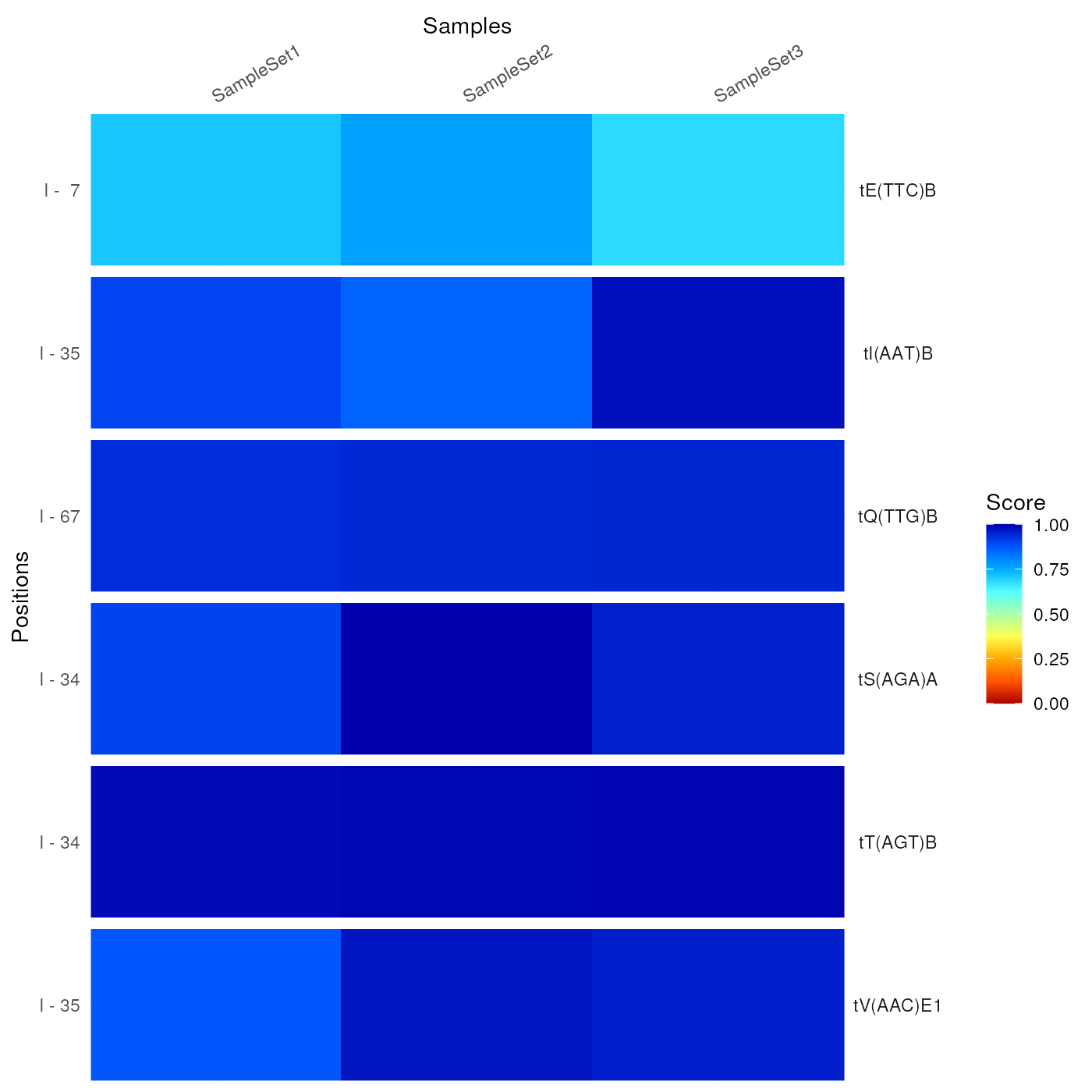
Heatmap for identified Inosine positions.
Additionally, the order of sample sets can be adjusted, normalized to any of the sample sets and the numbering of positions shown per transcript.
plotCompareByCoord(msi[c(3,1,2)], coord, alias = alias, normalize = "SampleSet3",
                   perTranscript = TRUE)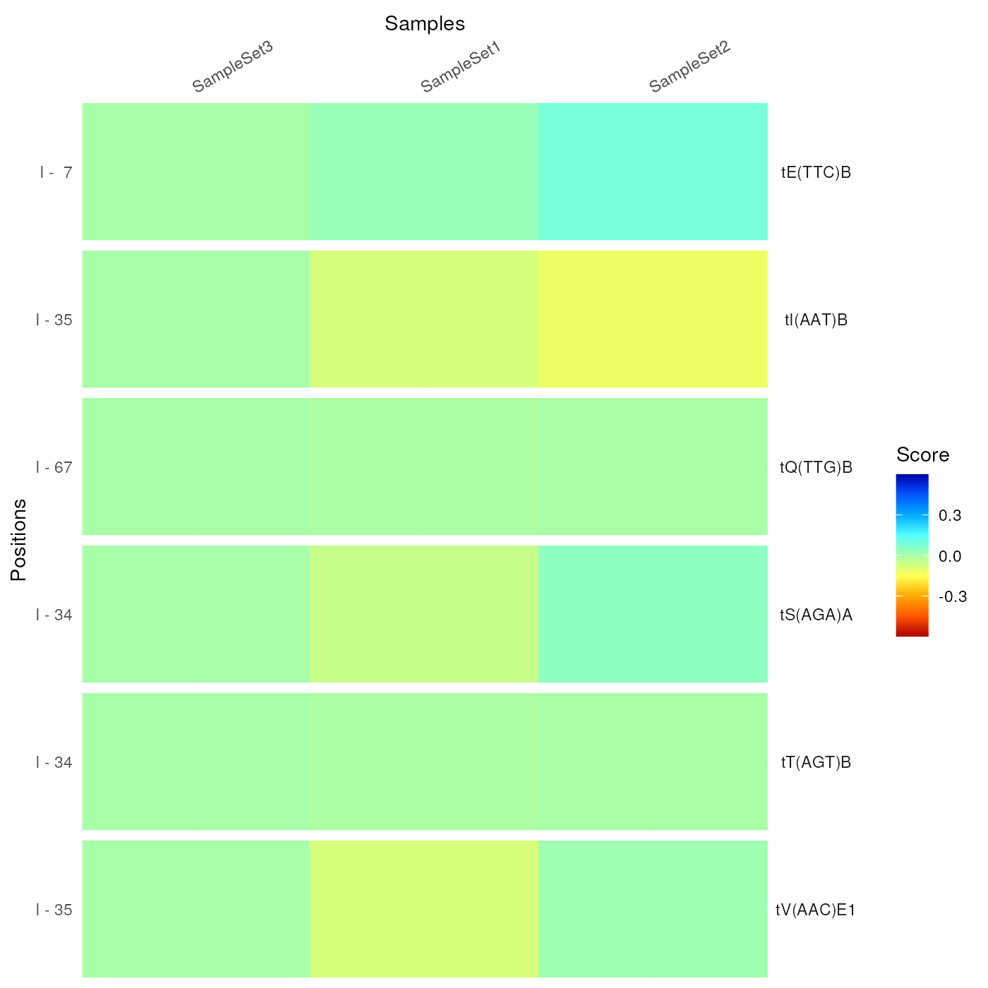
Heatmap for identified Inosine positions with normalized scores.
The calculated scores and data can be visualized along the
transcripts or chunks of the transcript. With the optional argument
showSequenceData the plotting of the sequence data in
addition to the score data can be triggered by setting it to
TRUE.
plotData(msi, "2", from = 10L, to = 45L, alias = alias) # showSequenceData = FALSE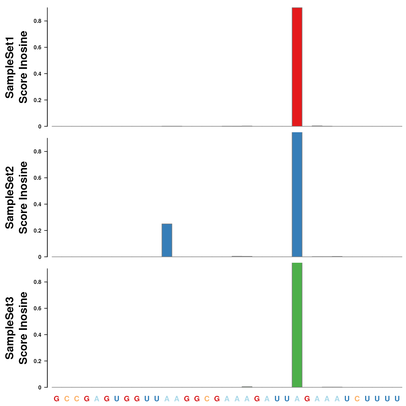
Scores along a transcript containing a A to G conversion indicating the presence of Inosine.
plotData(msi[1:2], "2", from = 10L, to = 45L, showSequenceData = TRUE, alias = alias)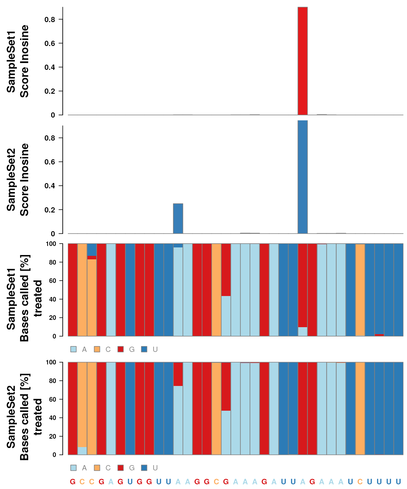
Scores along a transcript containing a A to G conversion indicating the presence of Inosine. This figure includes the detailed pileup sequence data.
Performance measurements
Since the detection of modifications from high throughput sequencing
data relies usually on thresholds for calling modifications, there is
considerable interest in analyzing the performance of the method based
on scores chosen and available samples. To analyse the performance, the
function plotROC() is implemented, which is a wrapper
around the functionality of the ROCR package Sing et al.
(2005).
For the example data used in this vignette, the information gained is
rather limited and the following figure should be regarded just as a
proof of concept. In addition, the use of found modifications sites as
an input for plotROC is strongly discouraged, since defeats
the purpose of the test. Therefore, please regard this aspect of the
next chunk as proof of concept as well.
plotROC(msi, coord)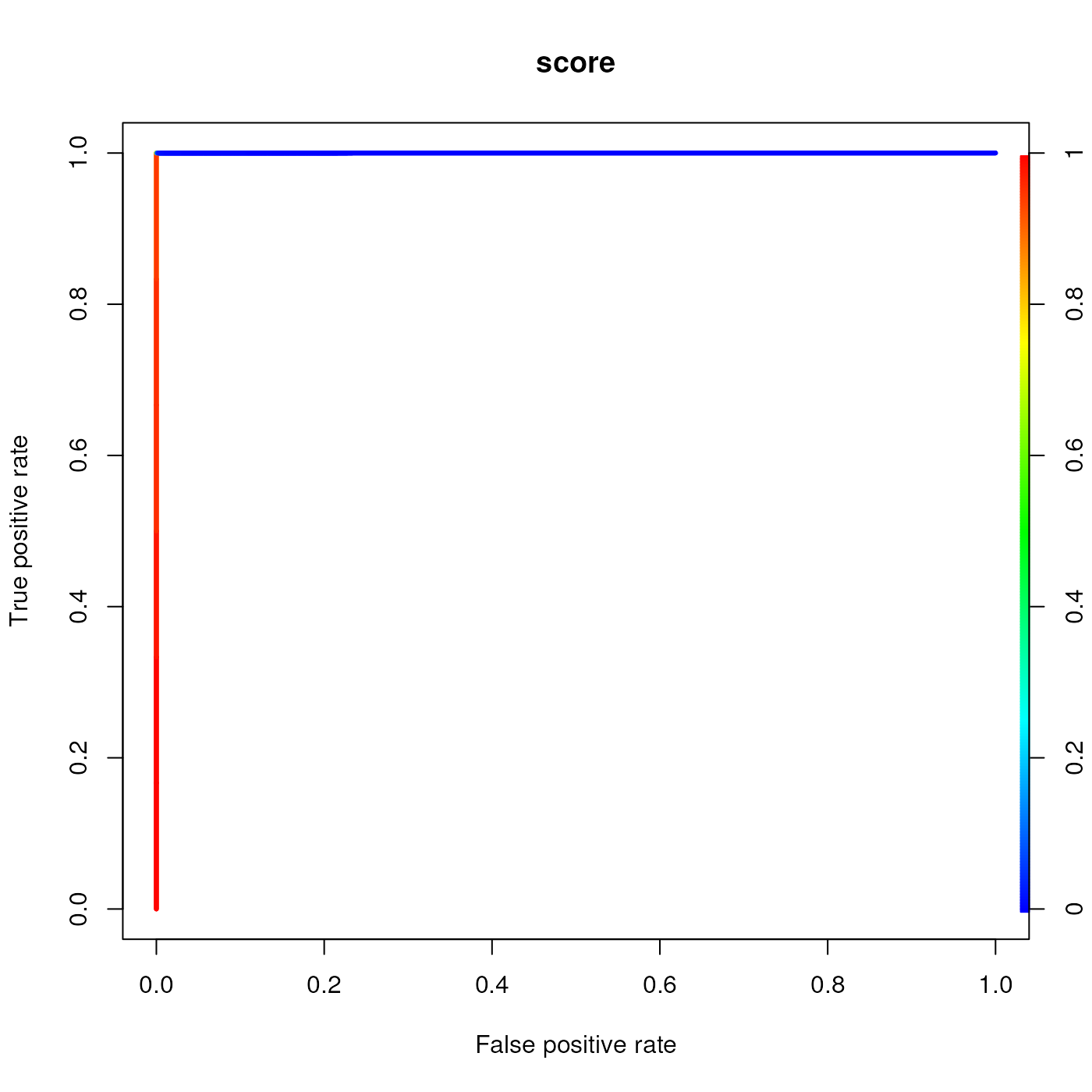
TPR vs. FPR plot.
Please have a look at ?plotROC for additional details.
Most of the functionality from the ROCR package is
available via additional arguments, thus the output of
plotROC can be heavily customized.
Additional informations
To have a look at metadata of reads for an analysis with
RNAmodR the function stats() can be used. It
can be used with a bunch of object types: SequenceData,
SequenceDataList, SequenceDataSet,
Modifier or ModifierSet. For
SequenceData* objects, the BamFile to be
analyzed must be provided as well, which automatically done for
Modifier* objects. For more details have a look at
?stats.
stats <- stats(msi)
stats
## List of length 3
## names(3): SampleSet1 SampleSet2 SampleSet3
stats[["SampleSet1"]]## DataFrameList of length 3
## names(3): treated treated treated
stats[["SampleSet1"]][["treated"]]## DataFrame with 12 rows and 6 columns
## seqnames seqlength mapped unmapped used used_distro
## <factor> <integer> <numeric> <numeric> <IntegerList> <List>
## 1 chr1 1800 197050 0 159782 83,1252,860,...
## 2 chr2 85 5863 0 2459 2,16,16,...
## 3 chr3 76 76905 0 63497 35,478,4106,...
## 4 chr4 77 8299 0 6554 6,27,36,...
## 5 chr5 74 11758 0 8818 520,105,93,...
## ... ... ... ... ... ... ...
## 8 chr8 75 144293 0 143068 14,44,48,...
## 9 chr9 75 13790 0 9753 1,49,43,...
## 10 chr10 85 19861 0 17729 35,21,10,...
## 11 chr11 77 10532 0 9086 53,92,185,...
## 12 * 0 0 961095 NA NAThe data returned by stats() is a
DataFrame, which can be wrapped as a
DataFrameList or a SimpleList depending on the
input type. Analysis of the data must be manually done and can be used
to produced output like the following plot for distribution of lengths
for reads analyzed.
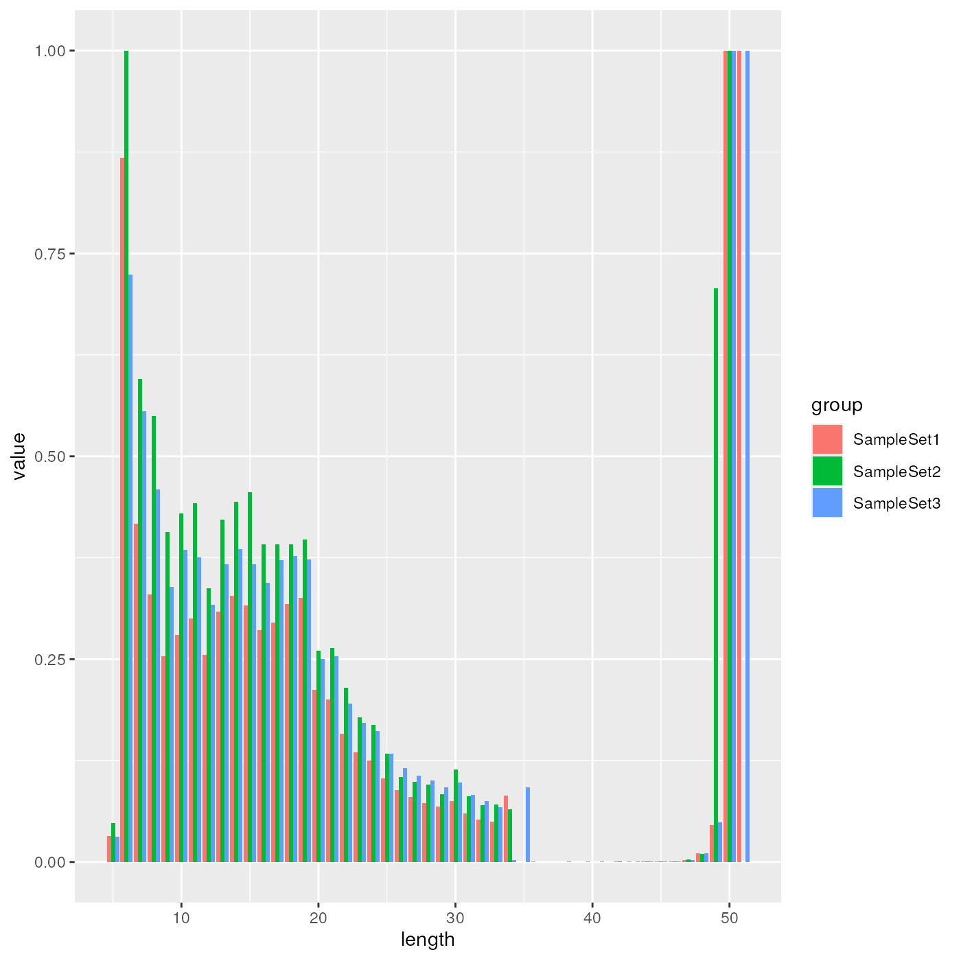
Distribution of lengths for reads used in the analysis
Further development
The development of RNAmodR will continue. General
ascpects of the analysis workflow will be addressed in the
RNAmodR package, whereas additional classes for new
sequencing techniques targeted at detecting post-transcriptional will be
wrapped in individual packages. This will allow general improvements to
propagate upstream, but not hinder individual requirements of each
detection strategy.
For an example have a look at the RNAmodR.RiboMethSeq
and RNAmodR.AlkAnilineSeq packages.

Features, which might be added in the future:
- interaction with our packages for data aggregation (for example meta gene aggregation)
- interaction with our packages for downstream analysis for visualization
We welcome contributions of any sort.
Sessioninfo
## R version 4.5.1 (2025-06-13)
## Platform: x86_64-pc-linux-gnu
## Running under: Ubuntu 24.04.3 LTS
##
## Matrix products: default
## BLAS:   /usr/lib/x86_64-linux-gnu/openblas-pthread/libblas.so.3
## LAPACK: /usr/lib/x86_64-linux-gnu/openblas-pthread/libopenblasp-r0.3.26.so;  LAPACK version 3.12.0
##
## locale:
##  [1] LC_CTYPE=en_US.UTF-8       LC_NUMERIC=C
##  [3] LC_TIME=en_US.UTF-8        LC_COLLATE=en_US.UTF-8
##  [5] LC_MONETARY=en_US.UTF-8    LC_MESSAGES=en_US.UTF-8
##  [7] LC_PAPER=en_US.UTF-8       LC_NAME=C
##  [9] LC_ADDRESS=C               LC_TELEPHONE=C
## [11] LC_MEASUREMENT=en_US.UTF-8 LC_IDENTIFICATION=C
##
## time zone: UTC
## tzcode source: system (glibc)
##
## attached base packages:
## [1] stats4    stats     graphics  grDevices utils     datasets  methods
## [8] base
##
## other attached packages:
##  [1] RNAmodR_1.23.2           Modstrings_1.25.0        RNAmodR.Data_1.23.0
##  [4] ExperimentHubData_1.35.0 AnnotationHubData_1.39.2 futile.logger_1.4.3
##  [7] ExperimentHub_2.99.5     AnnotationHub_3.99.6     BiocFileCache_2.99.6
## [10] dbplyr_2.5.1             txdbmaker_1.5.6          GenomicFeatures_1.61.6
## [13] AnnotationDbi_1.71.1     Biobase_2.69.1           Rsamtools_2.25.3
## [16] Biostrings_2.77.2        XVector_0.49.1           rtracklayer_1.69.1
## [19] GenomicRanges_1.61.4     Seqinfo_0.99.2           IRanges_2.43.2
## [22] S4Vectors_0.47.2         BiocGenerics_0.55.1      generics_0.1.4
## [25] BiocStyle_2.37.1
##
## loaded via a namespace (and not attached):
##   [1] RColorBrewer_1.1-3          rstudioapi_0.17.1
##   [3] jsonlite_2.0.0              magrittr_2.0.4
##   [5] farver_2.1.2                rmarkdown_2.29
##   [7] fs_1.6.6                    BiocIO_1.19.0
##   [9] ragg_1.5.0                  vctrs_0.6.5
##  [11] ROCR_1.0-11                 memoise_2.0.1
##  [13] RCurl_1.98-1.17             base64enc_0.1-3
##  [15] htmltools_0.5.8.1           S4Arrays_1.9.1
##  [17] BiocBaseUtils_1.11.2        progress_1.2.3
##  [19] lambda.r_1.2.4              curl_7.0.0
##  [21] SparseArray_1.9.1           Formula_1.2-5
##  [23] sass_0.4.10                 bslib_0.9.0
##  [25] htmlwidgets_1.6.4           desc_1.4.3
##  [27] plyr_1.8.9                  Gviz_1.53.1
##  [29] httr2_1.2.1                 futile.options_1.0.1
##  [31] cachem_1.1.0                GenomicAlignments_1.45.4
##  [33] lifecycle_1.0.4             pkgconfig_2.0.3
##  [35] Matrix_1.7-4                R6_2.6.1
##  [37] fastmap_1.2.0               BiocCheck_1.45.18
##  [39] MatrixGenerics_1.21.0       digest_0.6.37
##  [41] colorspace_2.1-2            OrganismDbi_1.51.4
##  [43] textshaping_1.0.3           Hmisc_5.2-3
##  [45] RSQLite_2.4.3               labeling_0.4.3
##  [47] filelock_1.0.3              colorRamps_2.3.4
##  [49] httr_1.4.7                  abind_1.4-8
##  [51] compiler_4.5.1              withr_3.0.2
##  [53] bit64_4.6.0-1               backports_1.5.0
##  [55] htmlTable_2.4.3             S7_0.2.0
##  [57] biocViews_1.77.4            BiocParallel_1.43.4
##  [59] DBI_1.2.3                   biomaRt_2.65.14
##  [61] rappdirs_0.3.3              DelayedArray_0.35.3
##  [63] rjson_0.2.23                tools_4.5.1
##  [65] foreign_0.8-90              nnet_7.3-20
##  [67] glue_1.8.0                  restfulr_0.0.16
##  [69] grid_4.5.1                  stringdist_0.9.15
##  [71] checkmate_2.3.3             reshape2_1.4.4
##  [73] cluster_2.1.8.1             gtable_0.3.6
##  [75] BSgenome_1.77.2             ensembldb_2.33.2
##  [77] data.table_1.17.8           hms_1.1.3
##  [79] BiocVersion_3.22.0          pillar_1.11.1
##  [81] stringr_1.5.2               dplyr_1.1.4
##  [83] lattice_0.22-7              deldir_2.0-4
##  [85] bit_4.6.0                   biovizBase_1.57.1
##  [87] tidyselect_1.2.1            RBGL_1.85.0
##  [89] knitr_1.50                  gridExtra_2.3
##  [91] bookdown_0.44               ProtGenerics_1.41.0
##  [93] SummarizedExperiment_1.39.2 xfun_0.53
##  [95] matrixStats_1.5.0           stringi_1.8.7
##  [97] UCSC.utils_1.5.0            lazyeval_0.2.2
##  [99] yaml_2.3.10                 evaluate_1.0.5
## [101] codetools_0.2-20            interp_1.1-6
## [103] tibble_3.3.0                BiocManager_1.30.26
## [105] graph_1.87.0                cli_3.6.5
## [107] rpart_4.1.24                systemfonts_1.2.3
## [109] jquerylib_0.1.4             Rcpp_1.1.0
## [111] dichromat_2.0-0.1           GenomeInfoDb_1.45.11
## [113] png_0.1-8                   XML_3.99-0.19
## [115] RUnit_0.4.33.1              parallel_4.5.1
## [117] pkgdown_2.1.3               ggplot2_4.0.0
## [119] blob_1.2.4                  prettyunits_1.2.0
## [121] jpeg_0.1-11                 latticeExtra_0.6-31
## [123] AnnotationFilter_1.33.0     AnnotationForge_1.51.0
## [125] bitops_1.0-9                VariantAnnotation_1.55.1
## [127] scales_1.4.0                purrr_1.1.0
## [129] crayon_1.5.3                rlang_1.1.6
## [131] KEGGREST_1.49.1             formatR_1.14