Genome-wide assessment of differential translations with ribosome profiling data the xtail package
Zhengtao Xiao
MOE Key Laboratory of BioinformaticsTsinghua-Peking Joint Center for Life SciencesSchool of Life Sciences, Tsinghua University, Beijing 100084, ChinaQin Zou
MOE Key Laboratory of BioinformaticsTsinghua-Peking Joint Center for Life SciencesSchool of Life Sciences, Tsinghua University, Beijing 100084, ChinaYu Liu
MOE Key Laboratory of BioinformaticsTsinghua-Peking Joint Center for Life SciencesSchool of Life Sciences, Tsinghua University, Beijing 100084, ChinaXuerui Yang
MOE Key Laboratory of BioinformaticsTsinghua-Peking Joint Center for Life SciencesSchool of Life Sciences, Tsinghua University, Beijing 100084, China2021-05-25
Source:vignettes/xtail.Rmd
xtail.RmdAbstract
If you use xtail in published research, please cite: Z. Xiao, Q. Zou, Y. Liu, X. Yang: Genome-wide assessment of differential translations with ribosome profiling data. Nat Commun 2016, 7:11194. http://www.ncbi.nlm.nih.gov/pubmed/27041671
Introduction
This package, Xtail, is for identification of genes undergoing differential translation across two conditions with ribosome profiling data. Xtail is based on a simple assumption that if a gene is subjected to translational dyresgulation under certain exprimental or physiological condition, the change of its RPF abundance should be discoordinated with that of mRNA expression. Specifically, xtail consists of three major steps: (1) modeling of ribosome profiling data using negative binomial distribution (NB), (2) estabilishment of probability distributions for fold changes of mRNA or RPF (or RPF-to-mRNA ratios), and (3) evaluation of statistical significance and magnitude of differential translations. The differential translation of each gene is evaluated by two pipelines: in the first one, xtail calculated the posterior probabilities for a range of mRNA or RPF fold changes, and eventually estabilished their probability distributions. These two distributions, represented as probability vectors, were then used to estabilish a joint probability distribution matrix, from which a new probability distribution were generated for differential translation. The P-values, point estimates and credible intervals of differential tranlsations were then calculated based on these results. In the other parallel pipline, xtail established probability distributions for RPF-to-mRNA ratios in two conditions and derived another distribution for differential translation. The more conserved set of results from these two parallel piplines was used as the final result. With this strategy, xtail performs quantification of differential translation for each gene, i.e., the extent to which a gene`s translational rate is not coordinated with the change of the mRNA expression.
By default, Xtail adapts the strategy of DESeq2 (Love, Huber, and Anders 2014) to normalize read counts of mRNA and RPF in all samples, and fits NB distributions with dispersions \(\alpha\) and \(\mu\).
This guide provides step-by-step instructions on how to load data, how to execute the package and how to interpret output.
Data Preparation
The xtail package uses read counts of RPF and mRNA, in the form of rectangular table of values. The rows and columns of the table represent the genes and samples, respectively. Each cell in the g-th row and the i-th columns is the count number of reads mapped to gene g in sample i.
Xtail takes in raw read counts of RPF and mRNA, and performs median-of-ratios normalization by default. This normalization method is also recommend by Reddy R. (Reddy 2015). Alternatively, users can provide normalized read counts and skip the built-in normalization in Xtail.
In this vignette, we select a published ribosome profiling dataset from human prostate cancer cell PC3 after mTOR signaling inhibition with PP242 (Hsieh et al. 2012). This dataset consists of mRNA and RPF data for 11391 genes in two replicates from each of the two conditions(treatment vs. control).
An example
Here we run xtail with the ribosome profiling data described above. First we load the library and data.
Next we can view the first five lines of the mRNA (mrna) and RPF (rpf) elements of xtaildata.
mrna <- xtaildata$mrna
rpf <- xtaildata$rpf
head(mrna,5)
## control1 control2 treat1 treat2
## ENSG00000000003 825 955 866 1039
## ENSG00000000419 1054 967 992 888
## ENSG00000000457 71 75 139 95
## ENSG00000000460 191 162 199 201
## ENSG00000000971 81 2 88 11
head(rpf,5)## control1 control2 treat1 treat2
## ENSG00000000003 143 302 197 195
## ENSG00000000419 234 481 383 306
## ENSG00000000457 12 17 17 15
## ENSG00000000460 45 88 63 37
## ENSG00000000971 31 7 36 2We assign condition labels to the columns of the mRNA and RPF data.
condition <- c("control","control","treat","treat")Next, we run the main function, xtail(). By default, the second condition (here is treat) would be compared against the first condition (here is control). Those genes with the minimum average expression of mRNA counts and RPF counts among all samples larger than 1 are used (can be changed by setting minMeanCount). All the available CPU cores are used for running program. The argument bins is the number of bins used for calculating the probability densities of log2FC and log2R. This paramater will determine accuracy of the final pvalue. Here, in order to keep the run-time of this vignette short, we will set bins to 1000. Detailed description of the arguments of the xtail function can be found by typing ?xtail at the R prompt.
test.results <- xtail(mrna,rpf,condition,bins=1000)## Calculating the library size factors## 1. Estimate the log2 fold change in mrna## 2. Estimate the log2 fold change in rpf## 3. Estimate the difference between two log2 fold changes## 4. Estimate the log2 ratio in first condition## 5. Estimate the log2 ratio in second condition## 6. Estimate the difference between two log2 ratios## Number of the log2FC and log2R used in determining the final p-value## log2FC: 2033## log2R: 9358Now we can extract a results table using the function `resultsTable}, and examine the first five lines of the results table.
test.tab <- resultsTable(test.results)
head(test.tab,5)
## DataFrame with 5 rows and 8 columns
## log2FC_TE_v1 pvalue_v1 treat_log2TE log2FC_TE_v2 pvalue_v2
## <numeric> <numeric> <numeric> <numeric> <numeric>
## ENSG00000000003 0.0586807 0.816556 0.5525063 0.0606827 0.809767
## ENSG00000000419 0.3559950 0.156433 1.3654645 0.3559950 0.142658
## ENSG00000000457 -0.2993342 0.590709 -0.0608568 -0.2961310 0.644911
## ENSG00000000460 -0.3108003 0.422875 0.8068549 -0.3109200 0.429114
## ENSG00000000971 -0.6223233 0.710533 1.2996842 -0.6457720 0.744394
## log2FC_TE_final pvalue_final pvalue.adjust
## <numeric> <numeric> <numeric>
## ENSG00000000003 0.0586807 0.816556 0.995279
## ENSG00000000419 0.3559950 0.156433 0.995279
## ENSG00000000457 -0.2961310 0.644911 0.995279
## ENSG00000000460 -0.3109200 0.429114 0.995279
## ENSG00000000971 -0.6457720 0.744394 0.995279The results of fist pipline are named with suffix \_v1, which are generated by comparing mRNA and RPF log2 fold changes: The element log2FC_TE_v1 represents the log2 fold change of TE; The pvalue_v1 represent statistical significance. The sencond pipline are named with suffix \_v2, which are derived by comparing log2 ratios between two conditions: log2FC_TE_v2, and pvalue_v2 are log2 ratio of TE, and pvalues. Finally, the more conserved results (with larger-Pvalue) was select as the final assessment of differential translation, which are named with suffix \_final. The pvalue.adjust is the estimated false discovery rate corresponding to the pvalue_final.
Users can also get the log2 fold changes of mRNA and RPF, or the log2 ratios of two conditions by setting log2FCs or log2Rs as TRUE in resultsTable. And the results table can be sorted by assigning the sort.by. Detailed description of the resultsTable function can be found by typing ?resultsTable.
Finally, the plain-text file of the results can be exported using the functions write.csv or write.table.
write.table(test.tab,"test_results.txt",quote=FALSE,sep="\t")We also provide a very simple function, write.xtail (using the write.table function), to export the xtail result (test.results) to a tab delimited file.
write.xtail(test.results, file = "test_results.txt", quote = FALSE, sep = "\t")Visualization
plotFCs
In Xtail, the function plotFCs shows the result of the differential expression at the two expression levels, where each gene is a dot whose position is determined by its log2 fold change (log2FC) of transcriptional level (mRNA_log2FC), represented on the x-axis, and the log2FC of translational level (RPF_log2FC), represented on the y-axis (Figure @ref(fig:plotFCs)). The optional input parameter of plotFCs is log2FC.cutoff, a non-negative threshold value that will divide the genes into different classes:
-
blue: for genes whoesmRNA_log2FClarger thanlog2FC.cutoff(transcriptional level). -
red: for genes whoesRPF_log2FClarger thanlog2FC.cutoff(translational level). -
green: for genes changing homodirectionally at both level. -
yellow: for genes changing antidirectionally at two levels.
plotFCs(test.results)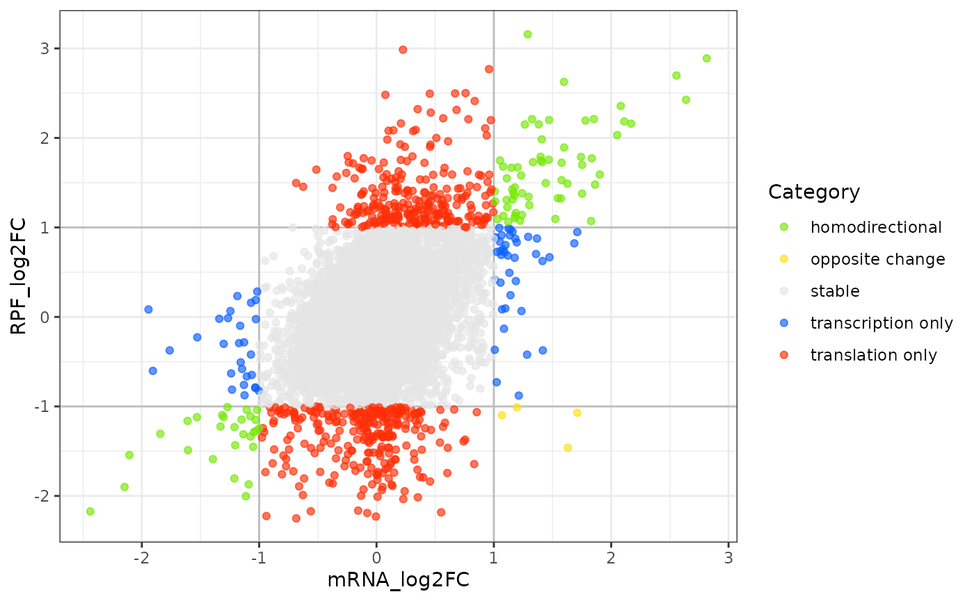
Scatter plot of log2 fold changes
Those genes in which the difference of mRNA_log2FC and RPF_log2FC did not exceed more than log2FC.cutoff are excluded. The points will be color-coded with the pvalue_final obtained with xtail (more significant p values having darker color). By default the log2FC.cutoff is 1.
plotRs
Similar to plotFCs, the function plotRs shows the RPF-to-mRNA ratios in two conditions, where the position of each gene is determined by its RPF-to-mRNA ratio (log2R) in two conditions, represented on the x-axis and y-axis respectively (Figure @ref(fig:plotRs)). The optional input parameter log2R.cutoff (non-negative threshold value) will divide the genes into different classes:
-
blue: for genes whoeslog2Rlarger in first condition than second condition. -
red: for genes whoeslog2Rlarger in second condition than the first condition. -
green: for genes whoeslog2Rchanging homodirectionally in two condition. -
yellow: for genes whoeslog2Rchanging antidirectionally in two conditon.
plotRs(test.results)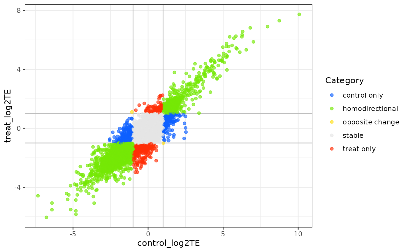
Scatter plot of log2 RPF-to-mRNA ratios
Those genes in which the difference of log2R in two conditions did not exceed more than log2R.cutoff are excluded. The points will be color-coded with the pvalue_final obtained with xtail (more significant p values having darker color). By default the log2R.cutoff is 1.
volcanoPlot
It can also be useful to evaluate the fold changes cutoff and p values thresholds by looking at the volcano plot. A simple function for making this plot is volcanoPlot, in which the log2FC_TE_final is plotted on the x-axis and the negative log10 pvalue_final is plotted on the y-axis (Figure @ref(fig:volcanoPlot)).
volcanoPlot(test.results)
volcano plot
Session info
## R version 4.0.3 (2020-10-10)
## Platform: x86_64-pc-linux-gnu (64-bit)
## Running under: Ubuntu 20.04 LTS
##
## Matrix products: default
## BLAS/LAPACK: /usr/lib/x86_64-linux-gnu/openblas-pthread/libopenblasp-r0.3.8.so
##
## locale:
##  [1] LC_CTYPE=en_US.UTF-8       LC_NUMERIC=C
##  [3] LC_TIME=en_US.UTF-8        LC_COLLATE=en_US.UTF-8
##  [5] LC_MONETARY=en_US.UTF-8    LC_MESSAGES=C
##  [7] LC_PAPER=en_US.UTF-8       LC_NAME=C
##  [9] LC_ADDRESS=C               LC_TELEPHONE=C
## [11] LC_MEASUREMENT=en_US.UTF-8 LC_IDENTIFICATION=C
##
## attached base packages:
## [1] parallel  stats4    stats     graphics  grDevices utils     datasets
## [8] methods   base
##
## other attached packages:
##  [1] xtail_1.2.0                 DESeq2_1.30.1
##  [3] SummarizedExperiment_1.20.0 Biobase_2.50.0
##  [5] MatrixGenerics_1.2.1        matrixStats_0.58.0
##  [7] GenomicRanges_1.42.0        GenomeInfoDb_1.26.7
##  [9] IRanges_2.24.1              S4Vectors_0.28.1
## [11] BiocGenerics_0.36.1         BiocStyle_2.18.1
##
## loaded via a namespace (and not attached):
##  [1] httr_1.4.2             bit64_4.0.5            splines_4.0.3
##  [4] assertthat_0.2.1       highr_0.8              BiocManager_1.30.10
##  [7] blob_1.2.1             GenomeInfoDbData_1.2.4 yaml_2.2.1
## [10] pillar_1.4.7           RSQLite_2.2.3          lattice_0.20-41
## [13] glue_1.4.2             digest_0.6.27          RColorBrewer_1.1-2
## [16] XVector_0.30.0         colorspace_2.0-0       htmltools_0.5.1.1
## [19] Matrix_1.3-2           pkgconfig_2.0.3        XML_3.99-0.5
## [22] genefilter_1.72.1      bookdown_0.21          zlibbioc_1.36.0
## [25] xtable_1.8-4           scales_1.1.1           BiocParallel_1.24.1
## [28] tibble_3.0.6           annotate_1.68.0        farver_2.0.3
## [31] ggplot2_3.3.3          ellipsis_0.3.1         cachem_1.0.4
## [34] survival_3.2-7         magrittr_2.0.1         crayon_1.4.1
## [37] memoise_2.0.0          evaluate_0.14          fs_1.5.0
## [40] textshaping_0.3.0      tools_4.0.3            lifecycle_1.0.0
## [43] stringr_1.4.0          locfit_1.5-9.4         munsell_0.5.0
## [46] DelayedArray_0.16.3    AnnotationDbi_1.52.0   compiler_4.0.3
## [49] pkgdown_1.6.1          systemfonts_1.0.1      rlang_0.4.10
## [52] grid_4.0.3             RCurl_1.98-1.2         labeling_0.4.2
## [55] bitops_1.0-6           rmarkdown_2.6          gtable_0.3.0
## [58] DBI_1.1.1              R6_2.5.0               knitr_1.31
## [61] fastmap_1.1.0          bit_4.0.4              rprojroot_2.0.2
## [64] ragg_1.1.0             desc_1.2.0             stringi_1.5.3
## [67] Rcpp_1.0.6             vctrs_0.3.6            geneplotter_1.68.0
## [70] xfun_0.21